The Programs barriers and treekin
Introduction
The following assumes you already have the barriers and treekin
programs installed. They are not part of the ViennaRNA Package
but their latest releases can be found at
https://www.tbi.univie.ac.at/RNA/Barriers/ and
https://www.tbi.univie.ac.at/RNA/Treekin/, respectively.
Installation proceeds as shown for the ViennaRNA Package.
Note
One problem that often occurs during treekin installation is the
dependency on blas and lapack packages. For further information
according to the barriers and treekin program also see the website.
A short recall on howto install/compile a program
Get the barriers source from https://www.tbi.univie.ac.at/RNA/Barriers/
extract the archive and go to the directory:
$ tar -xzf Barriers-1.5.2.tar.gz
$ cd Barriers-1.5.2
use the
--prefixoption to install in yourProgs/directory:$ ./configure --prefix=$HOME/Tutorial/Progs/barriers-1.5.2
make install:
$ make
$ make install
Now barriers is ready to use. Apply the same steps to install treekin.
Note
Copy the barriers and treekin binaries to your bin folder
or add the path to your PATH environment variable.
Calculate the Barrier Tree
$ echo UCCACGGCUGUUAGUGGAUAACGGC | RNAsubopt --noLP -s -e 10 > barseq.sub
$ barriers -G RNA-noLP --bsize --rates < barseq.sub > barseq.bar
You can restrict the number of local minima using the barriers
command-line option --max followed by a number. The option -G RNA-noLP
instructs barriers that the input consists of RNA secondary structures without
isolated basepairs. --bsize adds size of the gradient basins and --rates
tells barriers to compute rates between macro states/basins for use with
treekin. Another useful options is --minh to print only minima with
a barrier \(> dE\). Look at the output file barseq.bar, its content
should be like:
  UCCACGGCUGUUAGUGGAUAACGGC
1 (((((........))))).......  -6.90    0  10.00    115     0  -7.354207     23  -7.012023
2 ......(((((((.....)))))))  -6.80    1   9.30     32    58  -6.828221     38  -6.828218
3 (((...(((...)))))).......  -0.80    1   0.90      1    10  -0.800000      9  -1.075516
4 ....((..((((....)))).))..  -0.80    1   2.70      5    37  -0.973593     11  -0.996226
5 .........................   0.00    1   0.40      1    14  -0.000000     26  -0.612908
6 ......(((....((.....)))))   0.60    2   0.40      1    22   0.600000      3   0.573278
7 ......((((((....)))...)))   1.00    1   1.50      1    95   1.000000      2   0.948187
8 .((....((......)).....)).   1.40    1   0.30      1    30   1.400000      2   1.228342
The first row holds the input sequence, the successive list the local minima ascending in energy. The meaning of the first 5 columns is as follows
label (number) of the local minima (1=MFE)
structure of the minimum
free energy of the minimum
label of deeper local minimum the current minimum merges with (note that the
MFEhas no deeper local minimum to merge with)height of the energy barrier to the local minimum to merge with
numbers of structures in the basin we merge with
number of basin which we merge to
free energy of the basin
number of structures in this basin using gradient walk
gradient basin (consisting of all structures where gradientwalk ends in the minimum)
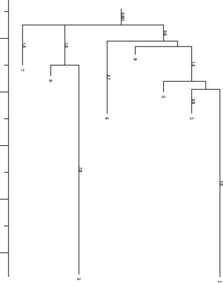
barriers produced two additional files, the PostScript file tree.eps
which represents the basic information of the barseq.bar file visually:

and a text file rates.out which holds the matrix of transition probabilities
between the local minima.
Simulating the Folding Kinetics
The program treekin is used to simulate the evolution over time of the
population densities of local minima starting from an initial population
density distribution \(p0\) (given on the command-line) and the transition
rate matrix in the file rates.out.
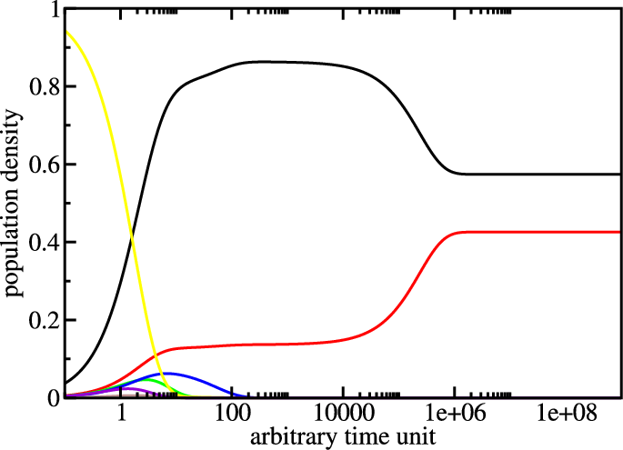
$ treekin -m I --p0 5=1 < barseq.bar | xmgrace -log x -nxy -
The simulation starts with all the population density in the open chain
(local minimum 5, see barseq.bar). Over time the population density of
this state decays (yellow curve) and other local minima get populated.
The simulation ends with the population densities of the thermodynamic
equilibrium in which the MFE (black curve) and local minimum 2 (red curve)
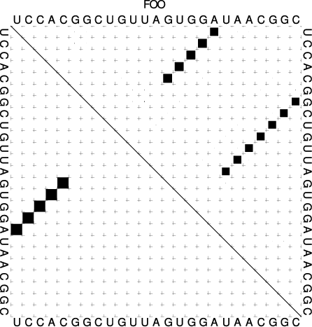
are the only ones populated. (Look at the dot plot of the sequence created
with RNAsubopt and RNAfold!)

