pair_style bop command
Syntax
pair_style bop keyword ...
- zero or more keywords may be appended
- keyword = save
save = pre-compute and save some values
Examples
pair_style bop
pair_coeff * * ../potentials/CdTe_bop Cd Te
pair_style bop save
pair_coeff * * ../potentials/CdTe.bop.table Cd Te Te
comm_modify cutoff 14.70
Description
The bop pair style computes Bond-Order Potentials (BOP) based on quantum mechanical theory incorporating both sigma and pi bondings. By analytically deriving the BOP from quantum mechanical theory its transferability to different phases can approach that of quantum mechanical methods. This potential is similar to the original BOP developed by Pettifor (Pettifor_1, Pettifor_2, Pettifor_3) and later updated by Murdick, Zhou, and Ward (Murdick, Ward). Currently, BOP potential files for these systems are provided with LAMMPS: AlCu, CCu, CdTe, CdTeSe, CdZnTe, CuH, GaAs. A sysstem with only a subset of these elements, including a single element (e.g. C or Cu or Al or Ga or Zn or CdZn), can also be modeled by using the appropriate alloy file and assigning all atom types to the singleelement or subset of elements via the pair_coeff command, as discussed below.
The BOP potential consists of three terms:
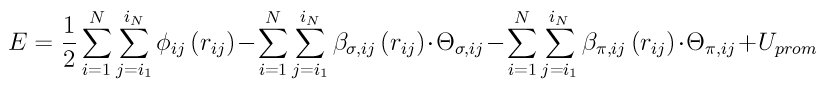
where phi_ij(r_ij) is a short-range two-body function representing the repulsion between a pair of ion cores, beta_(sigma,ij)(r_ij) and beta_(sigma,ij)(r_ij) are respectively sigma and pi bond ingtegrals, THETA_(sigma,ij) and THETA_(pi,ij) are sigma and pi bond-orders, and U_prom is the promotion energy for sp-valent systems.
The detailed formulas for this potential are given in Ward (Ward); here we provide only a brief description.
The repulsive energy phi_ij(r_ij) and the bond integrals beta_(sigma,ij)(r_ij) and beta_(phi,ij)(r_ij) are functions of the interatomic distance r_ij between atom i and j. Each of these potentials has a smooth cutoff at a radius of r_(cut,ij). These smooth cutoffs ensure stable behavior at situations with high sampling near the cutoff such as melts and surfaces.
The bond-orders can be viewed as environment-dependent local variables that are ij bond specific. The maximum value of the sigma bond-order (THETA_sigma) is 1, while that of the pi bond-order (THETA_pi) is 2, attributing to a maximum value of the total bond-order (THETA_sigma+THETA_pi) of 3. The sigma and pi bond-orders reflect the ubiquitous single-, double-, and triple- bond behavior of chemistry. Their analytical expressions can be derived from tight- binding theory by recursively expanding an inter-site Green’s function as a continued fraction. To accurately represent the bonding with a computationally efficient potential formulation suitable for MD simulations, the derived BOP only takes (and retains) the first two levels of the recursive representations for both the sigma and the pi bond-orders. Bond-order terms can be understood in terms of molecular orbital hopping paths based upon the Cyrot-Lackmann theorem (Pettifor_1). The sigma bond-order with a half-full valence shell is used to interpolate the bond-order expressiont that incorporated explicite valance band filling. This pi bond-order expression also contains also contains a three-member ring term that allows implementation of an asymmetric density of states, which helps to either stabilize or destabilize close-packed structures. The pi bond-order includes hopping paths of length 4. This enables the incorporation of dihedral angles effects.
Note
Note that unlike for other potentials, cutoffs for BOP potentials are not set in the pair_style or pair_coeff command; they are specified in the BOP potential files themselves. Likewise, the BOP potential files list atomic masses; thus you do not need to use the mass command to specify them. Note that for BOP potentials with hydrogen, you will likely want to set the mass of H atoms to be 10x or 20x larger to avoid having to use a tiny timestep. You can do this by using the mass command after using the pair_coeff command to read the BOP potential file.
One option can be specified as a keyword with the pair_style command.
The save keyword gives you the option to calculate in advance and store a set of distances, angles, and derivatives of angles. The default is to not do this, but to calculate them on-the-fly each time they are needed. The former may be faster, but takes more memory. The latter requires less memory, but may be slower. It is best to test this option to optimize the speed of BOP for your particular system configuration.
Only a single pair_coeff command is used with the bop style which specifies a BOP potential file, with parameters for all needed elements. These are mapped to LAMMPS atom types by specifying N additional arguments after the filename in the pair_coeff command, where N is the number of LAMMPS atom types:
- filename
- N element names = mapping of BOP elements to atom types
As an example, imagine the CdTe.bop file has BOP values for Cd and Te. If your LAMMPS simulation has 4 atoms types and you want the 1st 3 to be Cd, and the 4th to be Te, you would use the following pair_coeff command:
pair_coeff * * CdTe Cd Cd Cd Te
The 1st 2 arguments must be * * so as to span all LAMMPS atom types. The first three Cd arguments map LAMMPS atom types 1,2,3 to the Cd element in the BOP file. The final Te argument maps LAMMPS atom type 4 to the Te element in the BOP file.
BOP files in the potentials directory of the LAMMPS distribution have a ”.bop” suffix. The potentials are in tabulated form containing pre-tabulated pair functions for phi_ij(r_ij), beta_(sigma,ij)(r_ij), and beta_pi,ij)(r_ij).
The parameters/coefficients format for the different kinds of BOP files are given below with variables matching the formulation of Ward (Ward) and Zhou (Zhou). Each header line containing a ”:” is preceded by a blank line.
No angular table file format:
The parameters/coefficients format for the BOP potentials input file containing pre-tabulated functions of g is given below with variables matching the formulation of Ward (Ward). This format also assumes the angular functions have the formulation of (Ward).
- Line 1: # elements N
The first line is followed by N lines containing the atomic number, mass, and element symbol of each element.
Following the definition of the elements several global variables for the tabulated functions are given.
- Line 1: nr, nBOt (nr is the number of divisions the radius is broken into for function tables and MUST be a factor of 5; nBOt is the number of divisions for the tabulated values of THETA_(S,ij)
- Line 2: delta_1-delta_7 (if all are not used in the particular
- formulation, set unused values to 0.0)
Following this N lines for e_1-e_N containing p_pi.
- Line 3: p_pi (for e_1)
- Line 4: p_pi (for e_2 and continues to e_N)
The next section contains several pair constants for the number of interaction types e_i-e_j, with i=1->N, j=i->N
- Line 1: r_cut (for e_1-e_1 interactions)
- Line 2: c_sigma, a_sigma, c_pi, a_pi
- Line 3: delta_sigma, delta_pi
- Line 4: f_sigma, k_sigma, delta_3 (This delta_3 is similar to that of the previous section but is interaction type dependent)
The next section contains a line for each three body interaction type e_j-e_i-e_k with i=0->N, j=0->N, k=j->N
- Line 1: g_(sigma0), g_(sigma1), g_(sigma2) (These are coefficients for g_(sigma,jik)(THETA_ijk) for e_1-e_1-e_1 interaction. Ward contains the full expressions for the constants as functions of b_(sigma,ijk), p_(sigma,ijk), u_(sigma,ijk))
- Line 2: g_(sigma0), g_(sigma1), g_(sigma2) (for e_1-e_1-e_2)
The next section contains a block for each interaction type for the phi_ij(r_ij). Each block has nr entries with 5 entries per line.
- Line 1: phi(r1), phi(r2), phi(r3), phi(r4), phi(r5) (for the e_1-e_1 interaction type)
- Line 2: phi(r6), phi(r7), phi(r8), phi(r9), phi(r10) (this continues until nr)
- ...
- Line nr/5_1: phi(r1), phi(r2), phi(r3), phi(r4), phi(r5), (for the e_1-e_1 interaction type)
The next section contains a block for each interaction type for the beta_(sigma,ij)(r_ij). Each block has nr entries with 5 entries per line.
- Line 1: beta_sigma(r1), beta_sigma(r2), beta_sigma(r3), beta_sigma(r4), beta_sigma(r5) (for the e_1-e_1 interaction type)
- Line 2: beta_sigma(r6), beta_sigma(r7), beta_sigma(r8), beta_sigma(r9), beta_sigma(r10) (this continues until nr)
- ...
- Line nr/5+1: beta_sigma(r1), beta_sigma(r2), beta_sigma(r3), beta_sigma(r4), beta_sigma(r5) (for the e_1-e_2 interaction type)
The next section contains a block for each interaction type for beta_(pi,ij)(r_ij). Each block has nr entries with 5 entries per line.
- Line 1: beta_pi(r1), beta_pi(r2), beta_pi(r3), beta_pi(r4), beta_pi(r5) (for the e_1-e_1 interaction type)
- Line 2: beta_pi(r6), beta_pi(r7), beta_pi(r8), beta_pi(r9), beta_pi(r10) (this continues until nr)
- ...
- Line nr/5+1: beta_pi(r1), beta_pi(r2), beta_pi(r3), beta_pi(r4), beta_pi(r5) (for the e_1-e_2 interaction type)
The next section contains a block for each interaction type for the THETA_(S,ij)((THETA_(sigma,ij))^(1/2), f_(sigma,ij)). Each block has nBOt entries with 5 entries per line.
- Line 1: THETA_(S,ij)(r1), THETA_(S,ij)(r2), THETA_(S,ij)(r3), THETA_(S,ij)(r4), THETA_(S,ij)(r5) (for the e_1-e_2 interaction type)
- Line 2: THETA_(S,ij)(r6), THETA_(S,ij)(r7), THETA_(S,ij)(r8), THETA_(S,ij)(r9), THETA_(S,ij)(r10) (this continues until nBOt)
- ...
- Line nBOt/5+1: THETA_(S,ij)(r1), THETA_(S,ij)(r2), THETA_(S,ij)(r3), THETA_(S,ij)(r4), THETA_(S,ij)(r5) (for the e_1-e_2 interaction type)
The next section contains a block of N lines for e_1-e_N
- Line 1: delta^mu (for e_1)
- Line 2: delta^mu (for e_2 and repeats to e_N)
The last section contains more constants for e_i-e_j interactions with i=0->N, j=i->N
- Line 1: (A_ij)^(mu*nu) (for e1-e1)
- Line 2: (A_ij)^(mu*nu) (for e1-e2 and repeats as above)
Angular spline table file format:
The parameters/coefficients format for the BOP potentials input file containing pre-tabulated functions of g is given below with variables matching the formulation of Ward (Ward). This format also assumes the angular functions have the formulation of (Zhou).
- Line 1: # elements N
The first line is followed by N lines containing the atomic number, mass, and element symbol of each element.
Following the definition of the elements several global variables for the tabulated functions are given.
- Line 1: nr, ntheta, nBOt (nr is the number of divisions the radius is broken into for function tables and MUST be a factor of 5; ntheta is the power of the power of the spline used to fit the angular function; nBOt is the number of divisions for the tabulated values of THETA_(S,ij)
- Line 2: delta_1-delta_7 (if all are not used in the particular
- formulation, set unused values to 0.0)
Following this N lines for e_1-e_N containing p_pi.
- Line 3: p_pi (for e_1)
- Line 4: p_pi (for e_2 and continues to e_N)
The next section contains several pair constants for the number of interaction types e_i-e_j, with i=1->N, j=i->N
- Line 1: r_cut (for e_1-e_1 interactions)
- Line 2: c_sigma, a_sigma, c_pi, a_pi
- Line 3: delta_sigma, delta_pi
- Line 4: f_sigma, k_sigma, delta_3 (This delta_3 is similar to that of the previous section but is interaction type dependent)
The next section contains a line for each three body interaction type e_j-e_i-e_k with i=0->N, j=0->N, k=j->N
- Line 1: g0, g1, g2... (These are coefficients for the angular spline of the g_(sigma,jik)(THETA_ijk) for e_1-e_1-e_1 interaction. The function can contain up to 10 term thus 10 constants. The first line can contain up to five constants. If the spline has more than five terms the second line will contain the remaining constants The following lines will then contain the constants for the remainaing g0, g1, g2... (for e_1-e_1-e_2) and the other three body interactions
The rest of the table has the same structure as the previous section (see above).
Angular no-spline table file format:
The parameters/coefficients format for the BOP potentials input file containing pre-tabulated functions of g is given below with variables matching the formulation of Ward (Ward). This format also assumes the angular functions have the formulation of (Zhou).
- Line 1: # elements N
The first two lines are followed by N lines containing the atomic number, mass, and element symbol of each element.
Following the definition of the elements several global variables for the tabulated functions are given.
- Line 1: nr, ntheta, nBOt (nr is the number of divisions the radius is broken into for function tables and MUST be a factor of 5; ntheta is the number of divisions for the tabulated values of the g angular function; nBOt is the number of divisions for the tabulated values of THETA_(S,ij)
- Line 2: delta_1-delta_7 (if all are not used in the particular
- formulation, set unused values to 0.0)
Following this N lines for e_1-e_N containing p_pi.
- Line 3: p_pi (for e_1)
- Line 4: p_pi (for e_2 and continues to e_N)
The next section contains several pair constants for the number of interaction types e_i-e_j, with i=1->N, j=i->N
- Line 1: r_cut (for e_1-e_1 interactions)
- Line 2: c_sigma, a_sigma, c_pi, a_pi
- Line 3: delta_sigma, delta_pi
- Line 4: f_sigma, k_sigma, delta_3 (This delta_3 is similar to that of the previous section but is interaction type dependent)
The next section contains a line for each three body interaction type e_j-e_i-e_k with i=0->N, j=0->N, k=j->N
- Line 1: g(theta1), g(theta2), g(theta3), g(theta4), g(theta5) (for the e_1-e_1-e_1 interaction type)
- Line 2: g(theta6), g(theta7), g(theta8), g(theta9), g(theta10) (this continues until ntheta)
- ...
- Line ntheta/5+1: g(theta1), g(theta2), g(theta3), g(theta4), g(theta5), (for the e_1-e_1-e_2 interaction type)
The rest of the table has the same structure as the previous section (see above).
Mixing, shift, table tail correction, restart:
This pair style does not support the pair_modify mix, shift, table, and tail options.
This pair style does not write its information to binary restart files, since it is stored in potential files. Thus, you need to re-specify the pair_style and pair_coeff commands in an input script that reads a restart file.
This pair style can only be used via the pair keyword of the run_style respa command. It does not support the inner, middle, outer keywords.
Restrictions
These pair styles are part of the MANYBODY package. They are only enabled if LAMMPS was built with that package (which it is by default). See the Making LAMMPS section for more info.
These pair potentials require the newtion setting to be “on” for pair interactions.
The CdTe.bop and GaAs.bop potential files provided with LAMMPS (see the potentials directory) are parameterized for metal units. You can use the BOP potential with any LAMMPS units, but you would need to create your own BOP potential file with coefficients listed in the appropriate units if your simulation does not use “metal” units.
Default
non-tabulated potential file, a_0 is non-zero.
(Pettifor_1) D.G. Pettifor and I.I. Oleinik, Phys. Rev. B, 59, 8487 (1999).
(Pettifor_2) D.G. Pettifor and I.I. Oleinik, Phys. Rev. Lett., 84, 4124 (2000).
(Pettifor_3) D.G. Pettifor and I.I. Oleinik, Phys. Rev. B, 65, 172103 (2002).
(Murdick) D.A. Murdick, X.W. Zhou, H.N.G. Wadley, D. Nguyen-Manh, R. Drautz, and D.G. Pettifor, Phys. Rev. B, 73, 45206 (2006).
(Ward) D.K. Ward, X.W. Zhou, B.M. Wong, F.P. Doty, and J.A. Zimmerman, Phys. Rev. B, 85,115206 (2012).
(Zhou) X.W. Zhou, D.K. Ward, M. Foster (TBP).